Using ICONS- Conditional Formatting

When I started writing my Excel Driven Dashboard course a couple of years ago I really started appreciating a more visual approach to Excel.
Now I am always incorporating color and images into spreadsheets wherever possible.
So, to that end, I want to talk about icon sets in Excel and how they can be useful.
In the example, I am going to go through I have a column of units sales that is compared against budget and a variance column.
If you have more than a couple of rows, it is difficult to quickly identify your problem areas. You may be able to sort the variance column it but I think using conditional formatting is more useful and helps to convey a better picture of what is going on.

Here is my data.  Yes- everyone knows about my love of chai and lattes!

Column D shows the variance. In case you are wondering I used the accounting format as I like the parentheses around negatives rather than the minus sign which is a little more difficult to see (maybe I am just getting old??)

Anyway, this is a short list but it is still difficult to determine which products are doing well compared against budget.  Using conditional formatting and the associated icon sets will make it much clearer.

1.First, select the data in the Variance column (D4.D12)
2.Go to the Home ribbon and click on Conditional Formatting and select Icon Sets.
3.Scroll down to the bottom and select More Rules

4.Go down to Icon Style and select one you like. I personally prefer ones that displays well on paper as well as online.

So, I wanted a green check mark to display on all the positive variances where actual is better than budget, a yellow to display if there is no variance and a red x to display if the variance is negative so:

5. Select >= from the drop-down list, type 1 in the Value section and select Number from the Type drop-down.
6.In the second row, select >=from the drop-down list, type 0 in the Value section and select Number from the Type drop-down.
Yes- having a < or <= would be nice – who the heck programs this stuff anyway?

7.Click OK.

Voila – at a glance you can see where the problem areas are.

Now, you may find that too busy so you do have some options.

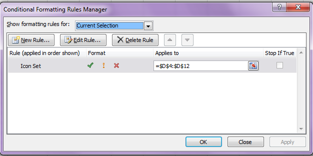
If you want to edit a Conditional Formatting rule – it is very easy – Select your data and  go back and click on Conditional Formatting and then select Manage Rules.

Click on Edit Rule…. 

Click and put an x in Show Icon only. This will hide the numbers and you will only see the icons.

An alternative if you want it clearer is to hide the green check marks so that you can focus on the problem products.
To do that, click on the drop-down beside the green check mark and select No Cell Icon from the top of the dialog box. You could also do this for the yellow exclamation if you were not concerned with products that made budget-barely.

Now, doesn’t this bottom screenshot look pretty clear and tell the story at a glance.

Now, I also like to see the numbers and even if I edit the rule and de-select Show Icons Only, it still looks messy so what I like to do is create an additional column and have the icons display there.  That way, I get the best of both worlds- the numbers and the visual impact.
So, I clicked in cell E4 and typed =D4 and then copied it down so I have the same numbers in Column D and E.
Then I selected Column E and did the steps 4-6 as outlined above and then clicked the Show Icons Only box and then selected No Cell Icon for the green check mark and the yellow exclamation point.  You have to admit this looks a lot cleaner.

Wow.. .time for that cup of coffee now!