Let’s start with SUBTOTAL().
There are 3 advantages of using the SUBTOTAL function rather than the icon.
- First, the subtotal function allows you to display the subtotal wherever you want it to display on the worksheet rather than in the list itself.
- Second, you can specify if you want Excel to subtotal all of the data in the list, even the hidden values, or to only subtotal the visible data in the list. That is powerful.
The syntax for SUBTOTAL is =SUBTOTAL(function_num, ref1,[ref2]…). The function_num indicates the mathematical operation you want Excel to do. For example, =Subtotal(1,B2:B50) tells Excel to Average the data in cells B2 through B50. Apparently the programmers sequenced the function_nums alphabetically rather than on frequency as you would normally expect that 1 would be to add – or at least I did. Anyway, I digress. 1 means to average, 2 to count and 9 means to sum. By using the single digit function_number, Excel automatically includes all hidden rows and columns in the list. If you use the corresponding 3 digit function_number, Excel subtotals only the visible list in the data. So, the function_num 1 includes the hidden rows, while 101 excludes them. Below is a list of the most common function_num:
- The third advantage of the Subtotal function is that it excludes other subtotals. So, for example, if you had a monthly report that has a lot of report sections such as Sales, Cost of Goods Sold, Operating Expenses, Non-Operating Gains(Losses) , typically you add up each grouping and then create a grand total. If you used =SUBTOTAL() on each of these groupings than all you need to do is use =SUBTOTAL() at the end of the report to get a grand total because SUBTOTAL() does not include subtotals when it totals! How cool is that? This is also a time saver if you need to create a new section for something new within the report as the grand total will automatically update if =SUBTOTAL() was used.
AGGREGATE()
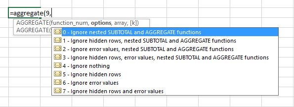
If you are excited about =SUBTOTAL() then check out =AGGREGATE() if you have Excel 2010 or higher. AGGREGATE() does everything that SUBTOTAL() does and more. While =SUBTOTAL() offers 11 functions, AGGREGATE() offers 19 functions. Some of the more useful new functions include SMALL() and LARGE(). In addition to offering you the option of ignoring hidden rows of data, it also allows you the option of ignoring error values and/or subtotals. This is key – how often have you tried to sum a column of data that has a #Div/0! Or a #N/A? Well, if you use AGGREGATE() you will actually get an answer instead of an error message in the total line.
The syntax of AGGREGATE() is similar to SUBTOTAL() but gives you more control over what you are totaling so it is more powerful.. It is AGGREGATE(function_num, options, ref1,[ref2],..]. A function_num of 1 still means Average while a 9 means Sum. The difference here is the options section. The option number tells Excel which values to ignore in the data list you are testing.
SUMMARY
So, why didn’t I lead with AGGREGATE()? I started with =SUBTOTAL() because a lot of people are familiar with the Subtotal Icon and it is a bit simpler. However, if you are a manager of lots of data, I suggest you jump over SUBTOTAL() and use AGGREGATE().
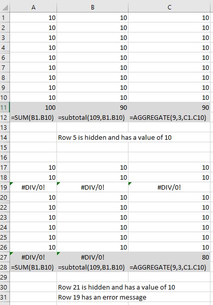
Below is a simple example comparing SUM(), SUBTOTAL(), AGGREGATE().


