I am in the process of updating my Pivot Table course and decided that I take another look at the GetPivotData function.
GET PIVOT DATA is an Excel function that pulls data from your pivot table. I personally don’t use it because if you hide a field you referenced in GETPIVOTDATA, the function stops working. Sometimes, just rearranging the fields in the table can impact the function as well. However, I did want you to be aware of it.
If you try to multiply a total in a pivot table, you will immediately see that Excel automatically references the GETPIVOTDATA function. This is a problem because if you copy the formula, you will get the same answer for the entire column or row.
In the example below, I opened Pivot_Rearrange.xlsx and removed the Product Name field from the Pivot Table. Next I clicked on cell C5, as I wanted to multiply B5 by 1.10 to estimate next year’s order amount by carrier.
Instead of showing =B5 it shows =GETPIVOTDATA(“Order Amount”,$A$3,”Ship Via”, “FedEx”)*1.10
Notice that A3 is treated as an absolute cell reference. If you copy the formula down, you will get the same answer for all of the Ship Via carriers. As a work around, I know many people who copy and paste the pivot table into another workbook if they want to do any math on the pivot table. However, I found a great tip on the MrExcel.com website on how to avoid this problem.
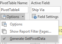
- Go up the Options icon and click the drop-down arrow to the right of it.
- Uncheck Generate GetPivotData.
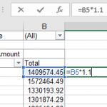
Now, if you go back to cell C5 and recreate the formula, you will see the formula bar now shows =B5*1.10. It will now copy down correctly. (Excel will not correct the GETPIVOTDATA formula so you need to delete it and then type in =B5*1.1.)
The best part is that once you uncheck it, Excel remembers so you do not have to keep unchecking the Generate GetPivotData icon every time you want to use a formula that references the pivot table.
This is an excerpt from my new Pivot Table Course that will be out the first week of June 2016.


