Formatting alternate Rows
Thanks to Diana Lawless for sending in this Excel tip.
Using the Shift key and the Format Painter icon together allows you to format an entire worksheet quickly. If you are formatting alternate rows or columns quickly and do want not mess around with Conditional formatting rules this is a great shortcut.
Diana wanted to format every other row of her 1,000+ row worksheet with a variety of formats to enhance readability.
To change formatting of the spreadsheet:
- Format line(s) as needed
- Highlight formatted line(s)
- Left click Format Painter (paintbrush)
- Hold ‘Shift’ key
- Tap ‘End’ key
- Tap down arrow key
- Release ‘Shift’ key
And voila! The formatting was automatically copied to every line in the spreadsheet.
If you have inserted new rows in an already formatted worksheet, this is a really quick way to fix any formatting problems.
Conditional Formatting and =MOD()
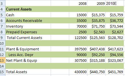
An alternative method, as mentioned above, is to use conditional formatting. If you use conditional formatting and the =MOD() function it is a quick way to create a general ledger type of effect with rows displayed in alternate colors.
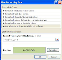
Below are the steps you can use to apply a rule to data. In my example here I am using the MOD function and telling Excel to shade every second row of my P&L so that it is easier to read. I am specifying 2 in the MOD function so that every second row is shaded and I am specifying green as that is the traditional accounting color but obviously you can select any color you want – just make sure that it is light enough that that the data can be seen through it.
1. Select your data
2. Click Conditional Formatting on the Home Ribbon.
3. Select New Rule.
4. Click on Use a Formula to determine which cells to format.
5. In the rule description, type =MOD(row(),2)=0.
6. Click Format.
7. Select a light green fill – this is usually associate with accounting general ledgers.
8. Click OK.
9. Click OK.
It should look something like the image below. It really does improve readability.

general ledger formatingt with =MOD

