Computing the Periodic Payment for a Loan
Excel Financial Function
Computing the periodic payment is probably the most used Excel financial function simply because it is something everyone uses.
Let’s walk through an example.
You want to purchase a car and finance $24,000 over 24 months at an interest rate of 4%. So, the question is –What is the monthly payment?
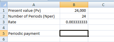
Here we have a value today (Pv) of $24,000. We want a monthly payment for 24 months (Nper) at an annual interest rate of 4%.
First, we need to change the annual interest rate to a monthly one by dividing 4% by 12 = .0033333 Let’s reflect this in our worksheet.
Matching the rate to the payment frequency is important. If you want to compute a monthly payment and have an annual rate, the rate must be divided by 12. (So many people forget this little fact which is why I am really emphasizing it here.)

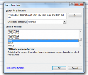
Click on cell B5, then click on the Fx button at the top left of the formulas tab.
At the top of the window that opens, select the category “Financial”, then find and select PMT at the bottom.

Click OK.

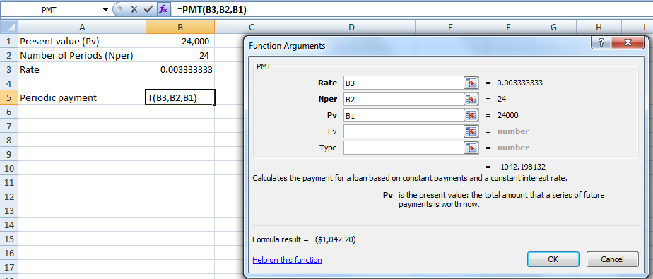
Fill in the cell references for Rate, Nper and PV as shown below: Rate is B3, Nper is B2 and PV is B1.
Click OK.
The monthly payment is $1,042.20. Remember, since this was a monthly payment, the annual interest rate was adjusted by dividing it by 12.Also, please note that the answer is negative as it is considered an outflow. Yes- you can tell the programmer was not a CPA 🙂 The easiest way to fix this is to go up to the formula bar and put a negative sign in front of PMT so that it looks like =-PMT(B3,B2,B1)
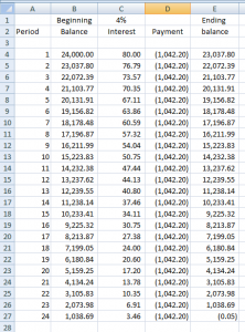
Let’s double-check our work by making an amortization schedule.
An amortization schedule starts with the initial loan amount and progresses it forward using the monthly interest rate and computed monthly payment.
Start with the beginning balance of $24,000. Add interest to this amount at 4% divided by 12 (=B1*.04/12). Reflect the payment as a negative amount and sum across the row (B4:D4) for the ending balance.

The new beginning balance in B5 should be the result in E4 (the formula in B5 will be =E4). Copy these down 23 rows (for a total of 23 periods). The ending balance should be very close to zero, but may not be exactly zero due to rounding (the use of only two decimal points in the payment).

This proves that the monthly payment for a loan of $24,000 over 24 months is correct and provides us with the interest and remaining balance at the end of each payment period.
Mortgages work identically except that the number of periods is generally longer.
