The AGGREGATE Function

The AGGREGATE function is a very powerful function for summarizing an array of data.
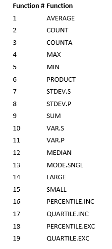
It combines 19 different ways to summarize data into one function!
While it is a powerful function, my favorite reason for using AGGREGATE is its ability to SUM data with errors. 

The syntax for the AGGREGATE function is =AGGREGATE(function #, options, array).
The function #’s are listed below:
/courses/

 

 

 

 

 

 

 

 

 

 

 

 

 

 

 

 

 

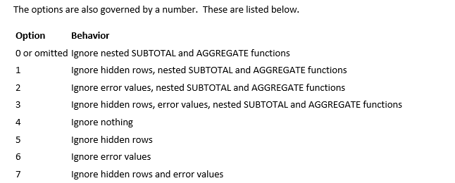
As you can see, your options permit you to ignore nested subtotals, hidden rows as well as error values.
One of my biggest pet peeves is trying to sum data that has error values.  The AGGREGATE function makes this easy.
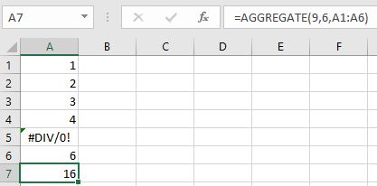
Assume you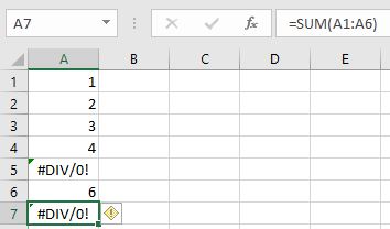 have data in cell A1:A6, and that you want to sum it.
However, because there is an error value in A5, the SUM function will return an error as shown in the screenshot on the left.
You can easily work around this by using the AGGREGATE function.

 

 

In this example, I clicked in A7 and  typed =AGGREGATE(

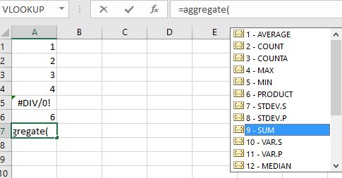
• A list of the various function #’s appears.  Note that if you elect to use the Insert Function dialog box, this handy list of functions does not appear.  We want to SUM the data, so function # 9 should be used, followed by a comma.

 

 

• After the comma, a list of options is presented.
• In this case, use option number 6, Ignore error values and place a comma after this.

 

 

 

 

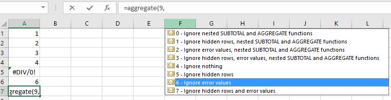
• Lastly, identify the array to be summed.  This will be accomplished by using the cursor to highlight A1:A6.
• Close the parenthesis.
• Press Enter.

 

 

 

 

 

 

The “Must Know” component of the AGGREGATE function is how to SUM data with errors.  It is a very powerful function, though.  You may find other uses for it in your professional assignments.

 

This is an excerpt from “Must Know Functions for CPAs”.